Normal distribution
For all our statistics, our dependent variable needs to be normally distributed, or have a normal distribution. You may have also heard it called a bell-shaped curve. It has really important statistical properties which is why most of the inferential statistics we’ll be learning in this class are parametric statistics that assume our data has a normal distribution.
Some of the important statistical properties of the normal distribution:
Data are equally distributed on both sides of the mean.
Skew and kurtosis are equal to 0, which is to say there is no skew or bad kurtosis.
The mean is equal to the median, and both are the exact center of the distribution of data. In other words, if your mean and median are not the same, you know you have skewed data! In fact, if your median < mean then you have positive skew and if your median > mean then you have negative skew.
We know the percentage of cases within 1, 2, 3, etc. standard deviations from the mean.
There are four ways to test for normality and we should test for normality using as many tests as we possibly can!
- Visualize the distribution
- Test the skew and kurtosis
- Conduct a Shapiro-Wilk test
- Visualize the Q-Q plot
Visualize the distribution
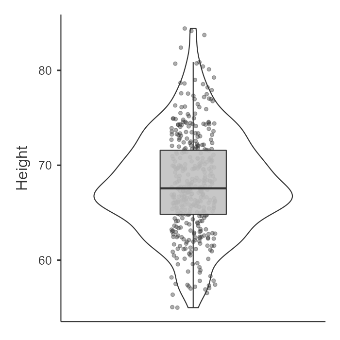
In jamovi, we can go to the Explorations option and choose Descriptives. Under Plots, we can choose a histogram and/or density plot (figure on the left) or boxplot and/or violin plot and/or data points (figure on the right). We can just look at this data and visually inspect with our eyes whether the data is normally distributed based on the density curve. We are looking to see to what extent it looks like a normal distribution. Height looks pretty fairly normally distributed in this case.

Test the skew and kurtosis
In jamovi, we can go to the Explorations option and choose Descriptives. Under statistics, choose skew and kurtosis. You’ll have to do a bit more work to actually figure out whether the skew and kurtosis is problematic though.
For height, here is our skew and kurtosis:
| Descriptives | Height |
| Skewness | .230 |
| Std. error skewness | .121 |
| Kurtosis | .113 |
| Std. error kurtosis | .241 |
We need to calculate z-scores for skew and kurtosis. We do that by dividing the value by its standard error:
Skew: .230 / .121 = 1.90
Kurtosis: .113 / .241 = .47
How do we know if it’s problematic? If the z-score for skew or kurtosis are less than |1.96| then it is not statistically significant and is normally distributed. However, if the z > |1.96| then it is statistically significant and is not normally distributed. In this case, both skew and kurtosis z-scores are less than 1.96 so we meet the assumption of normal distribution as evidenced by skew and kurtosis.
Shapiro-Wilk test
In jamovi, we can go to the Explorations option and choose Descriptives. Under statistics, choose Shapiro-Wilk. It will provide you the Shapiro-Wilk W test statistic and its respective p-value. In our case, Shapiro-Wilk’s for height is 68.03, p = .070. If the Shapiro-Wilk’s test is not statistically significant then it is normally distributed. However, if the Shapiro-Wilk’s test is statistically significant then it is not normally distributed. In this case, our Shapiro-Wilk’s test is not statistically significant so we meet the assumption of normal distribution as evidenced by the Shapiro-Wilk’s test.
Q-Q plot
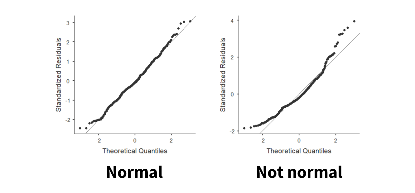
Last, we can visualize the Q-Q plot. In jamovi, we can go to the Explorations option and choose Descriptives. Under plots, choose Q-Q plot. We don’t need to go into details of what is being visualized, but what we are looking for is that the data points fall along the diagonal line. On the figure on the left, we can see that the data is pretty well falling on the diagonal line (with small deviations at the tails) so we can say it looks normally distributed. However, on the figure on the right, the data points deviate from the diagonal line pretty significantly and so we can say it does not look normally distributed.
Remember we should look at all pieces of evidence to determine whether we meet the assumption of normal distribution. Typically, all four will support each other, but there are times when some evidence contradicts other evidence. You’ll have to use your best judgment there, and often the visual inspection is the one I prioritize (e.g., if it doesn’t look normally distributed but then the other tests suggest it is, I would probably be cautious and just say we don’t meet the assumption).
Here’s a video by Alexander Swan on interpreting a Q-Q plot in jamovi: