4.1 An example of hypothesis testing
Imagine a researcher wants to replicate Alburt Bandura’s famous Bobo doll experiment. In this study, the researcher randomly assigns 30 six-year-old children to one of two conditions: one group watches a video of an adult showing aggressive behavior toward a Bobo doll and the other group watches a video of an adult passively playing with a Bobo doll. After watching their assigned video, children then went to the same room from the videos with the same Bobo doll. Researchers observed for aggressive behaviors6.
4.1.1 1. Write your hypotheses
The first step is to write out our hypotheses. We need to write our alternative and null hypotheses.
The alternative hypothesis is typically what we expect the results of the study to be. We often expect to see something; that there is an effect. We usually write this out as H1.
The null hypothesis is typically what we don’t expect the results of the study to be. It is often that there was no effect of the study. We usually write this out as H0.
The two hypotheses–our alternative and null hypotheses–must be mutually exclusive and exhaustive. Mutually exclusive means a potential result of the study cannot support both the alternative and null hypothesis; it must exclusively support only one. Exhaustive means the entire possible universe of results must be captured in our two hypotheses; it must exhaust all possible results.
We might also have directional or non-directional hypotheses. Directional hypotheses are also called one-tailed hypotheses because only one tail of the distribution would lead us to fail to reject the null hypothesis. Non-directional hypotheses are such that we don’t know whether the difference will be greater or less than 0, but we just think there will be a difference; these are also called two-tailed hypotheses because both tails of the distribution would lead us to fail to reject the null hypothesis. This will make a little more sense below and a lot more sense in the next chapter.
What might the hypotheses be for our example study? There should be theory and research to support alternative hypotheses. There is ample research now that viewing aggression leads to aggression through imitation and observed learning. Therefore, the researcher likely has a hypothesis that watching the aggressive adult will lead to more aggressive behavior than watching the passive adult.
Therefore, our hypotheses would be:
H1: Children watching the video with the adult aggressively playing with the Bobo doll will exhibit more aggressive behaviors than children watching the video with the adult playing passively.
H0: There will be no difference in children’s aggressive behaviors between the two groups or children watching the video with the adult aggressively playing with the Bobo doll will exhibit fewer aggressive behaviors than children watching the video with the adult playing passively.
Note that we now satisfy mutual exclusivity (no possible overlap in the hypotheses) and exhaustiveness (all possible results are captured).
A common error in a directional hypothesis like this is to forget that the null hypothesis is both no difference and the opposite. In other words, we have three possible options for our null and alternative hypotheses based on direction (\(\mu\) is the Greek letter “mu” and we often use it to signify the mean):
| Two-tailed | One-tailed (greater) | One-tailed (less than) | |
|---|---|---|---|
| Alternative (H1) | \(\mu_1\) != \(\mu_2\) | \(\mu_1\) > \(\mu_2\) | \(\mu_1\) < \(\mu_2\) |
| Null (H0) | \(\mu_1\) == \(\mu_2\) | \(\mu_1\) <= \(\mu_2\) | \(\mu_1\) >= \(\mu_2\) |
Since we’re talking about mean differences, we could also reformulate the above table slightly differently:
| Two-tailed | One-tailed (greater) | One-tailed (less than) | |
|---|---|---|---|
| Alternative (H1) | \(\mu_{diff}\) != 0 | \(\mu_{diff}\) > 0 | \(\mu_{diff}\) < 0 |
| Null (H0) | \(\mu_{diff}\) == 0 | \(\mu_{diff}\) <= 0 | \(\mu_{diff}\) >= 0 |
Note: != means “not equal” like the ≠ symbol. I write != because that is the notation that R uses for “not equal.”
Similarly, you might be wondering why I use == instead of just =. Again, this is the notion R uses for “exactly equal to.” In R, a single equal sign is usually equivalent to the assignment operator (e.g., x = 10 means assign 10 to the variable x).
4.1.2 2. Set the criteria for a decision
Our hypotheses simply state “more aggressive” or “no difference/less aggressive.” What constitutes more? What constitutes no difference? We have to specify that.
No difference seems easy. That’s a difference of zero, right? Well, not exactly, because it’s highly unlikely we would get an exact difference of zero. Therefore the question is: which values are close enough to a difference of zero that we’d still say that there is no difference? If our values are within that range, then we would fail to reject the null hypothesis. If our values are outside that range, then we would reject the null hypothesis.7
Let’s try to visualize this. We are saying that the null hypothesis is there is no difference (or less aggression), but at some point no difference turns into greater difference. Furthermore, we have a directional hypothesis in that we do not think the difference will be negative, that children watching the adult play aggressively will exhibit fewer aggressive behaviors. Basically, we need to know what the critical value is in the figure below.
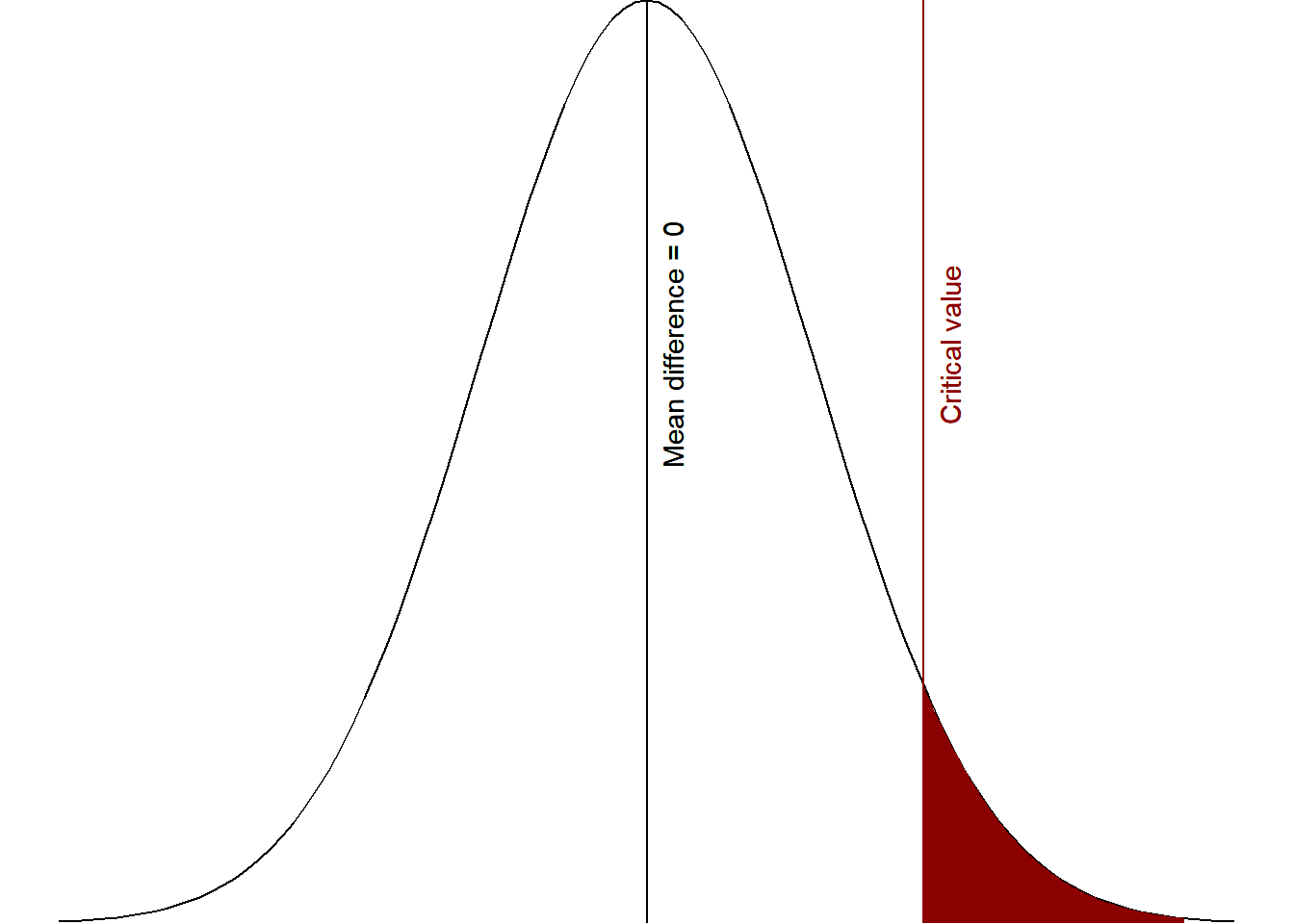
Figure 4.1: Critical area of statistical significance
We figure out that critical value based on what we set as our level of significance, also known as the alpha level. Most studies you read use the arbitrary \(\alpha\) = .05 (5%), although we really should be thinking critically about what alpha level we use (more on that in the next chapter). In the visualization above, we set the alpha to 5% and so the area shaded in red is exactly 5% of the area under the curve of the normal distribution.
Our alpha is the level of which we are saying would be considered “surprising” versus “not surprising.” If we got a mean difference that fell in that red area, then we would consider that “surprising” if we believed the null hypothesis was true. Basically, if we assume there is a mean difference of 0 (i.e., the null hypothesis), values past the critical value would be considered surprising enough that we would say that we reject the null hypothesis. This is why it is called null hypothesis significance testing.
In other words, the area in red are values that are unlikely to occur if the null hypothesis (in this case, mean difference <= 0) were true.
Now that we understand that a bit better, how do we find out our critical region? We do so based on our understanding of the incredible properties of the normal distribution! Back in the day before computers, some fancy mathematicians and statisticians figured out the exact t-values based on things like the direction of our hypothesis, our alpha, and our degrees of freedom. Let’s figure these out for our example:
- Direction of our hypothesis: we have already determined we’re using a one-tailed hypothesis.
- Alpha: let’s just go with \(\alpha\) = .05 for now
- Degrees of freedom: This is calculated by N - 2. We have 30 children total, so 30 - 2 is 28.
We then go to a t-value table like this one and find the cell we are looking for to identify our critical t-value (tcrit). First, our one-tailed probability is .05 so we’re going to look under the sixth column (t.95, one-tail = .05, two-tails = .10). Then we need to find the row for our degrees of freedom (df = 28). That leads us to a tcrit of 1.701.
Therefore, we can now finalize this step. Our criteria for decision is as such:
tobt > tcrit means we reject the null hypothesis.
tobt < tcrit means we fail to reject the null hypothesis
4.1.3 3. Perform the test statistic
We haven’t learned how to calculate the test statistic yet, but no worries we will get there soon. We had 30 participants, 15 in each condition. The researcher performed the experiment and got the following results:
Children who watched the video of the adult playing aggressively with the Bobo doll displayed an average of 51.10 aggressive behaviors (SD = 3.50).
Children who watched the video of the adult playing passively with the Bobo doll displayed an average of 27.40 aggressive behaviors (SD = 3.30).
That means the mean difference is 51.10 - 27.40 = 23.70. We’ll learn how to conduct a t-test later, but for now you can just input the numbers into this calculator. It nicely gives you a lot of the values, but the one we are looking for is the test statistic, which is tobt = 19.08 (notice we round to two decimals). It also gives us our p-values based on the null hypothesis, which in our case is that population 1 < population 2. The p-value is < .00001 but we never go to so many decimals, so we would say p < .001. The probability of getting a t-value as large as we did it less than .1% (less than our alpha of .05, so it is statistically significant). Very surprising!
4.1.4 4. Interpret results and draw a conclusion.
When tobt > tcrit we reject the null hypothesis which means our results are statistically significant (if our alpha is set to .05, then that means p < .05).
On the other hand, when tobt < tcrit we fail to reject the null hypothesis which means our results are not statistically significant (if our alpha is set to .05, then that means p > .05).
Since 19.08 > 1.701, we reject the null hypothesis that there is no difference in conditions or that children in the passive condition displayed more aggression than children in the aggressive condition.
However, this is when Type 1 and Type 2 errors come into play. Just because we get a result does not automatically mean that result is 100% accurate. There are many things that could lead us to an inaccurate interpretation!
I like to use this table when discussing errors. On the far left column, we have our results: were they statistically significant (p < .05) or not (p > .05)? On the top row, we have whether in the real world the null or alternative hypothesis is true. In reality, we can never truly know whether the null or alternative hypothesis is true. We can at best approximate our understanding of the real world through replication!
| H0 is true | H1 is true | |
|---|---|---|
| p < .05 (statistically significant) | Type 1 error | Correct interpretation |
| p > .05 (statistically non-significant) | Correct interpretation | Type 2 error |
Therefore, any time we get a statistically significant result (p < .05), then either we made a correct interpretation or we made a Type 1 error!
Similarly, any time we get a statistically non-significant results (p > .05) then either we made a correct interpretation or we made a Type 2 error!
A common mistake is assuming that p < .05 means that the alternative hypothesis is true. This is inaccurate because the p-value is the probability of our data given the null hypothesis is true. It says nothing about the alternative hypothesis. Similarly, a common mistake is assuming p > .05 means the alternative hypothesis is false. This is incorrect for the same exact reason.
Next week we’ll learn a lot more about p-values, errors, and more. For now, tuck this piece of information into your brain to remember!
4.1.5 Final note
When you read journal articles, you’ll note that they rarely discuss the null or alternative hypothesis. They may explain their research questions or their hypotheses (these hypotheses are their alternative hypotheses), but they rarely discuss the null.
This is not necessarily a bad thing. Rather, what may be problematic with it is if researchers apply NHST without critically thinking about what their null hypothesis is or whether they have a one-sided hypothesis, which leads researchers to use defaults when the defaults may not be most appropriate. However, it would probably be a better thing if everyone clearly specified their alternative and null hypotheses if they are doing NHST.
If you want to read more, this is a short read on the history of the .05 alpha level: https://www2.psych.ubc.ca/~schaller/528Readings/CowlesDavis1982.pdf↩︎
Note my language carefully here: fail to reject the null hypothesis OR reject the null hypothesis. Note how I am not saying support the alternative hypothesis! Through null hypothesis significance testing, we are only ever testing the null hypothesis and therefore can only make conclusions about it. This is why we need replication studies to provide ample support for alternative hypotheses.↩︎